ACPY
ACPy is an auto-calibration utility for GOTM and fabm0d . ACPy is written in Python.
Introduction
The calibration of complex coupled physical/bio-geochemical numerical models is a very time-consuming task typical requiring a large number of - run model -> compare with observations -> adjust paramters - cycles. The final chosen set of model parameters is the - partly - subjective judgement by the person performing the calibration and do not in anyway assure that even a small part of the global parameter space has been covered. This is mainly due to the curse of dimensionality stating that the number of tries becomes so large that it is impossible due to resource limitations on todays computers. As an example - with only 3 model parameters and 10 subdivisions in each paramter space 1000 simulations are needed if a brute force method is applied. For models counting 10’s to 100’s a systematic search of the optimal set of parameters in the full space is impossible.
The problem sketched above is by no means unique to the field of numerical models of natural waters and a lot of research has been done during the last decades. As it is not possible to guarantee the optimal solution statistical methods have been developed. Many of these methods are based on Monte Carlo methods - i.e. a statistical method where the optimal solution is based on a choice between a number of tries. The optimal choice is based on the evaluation of an objective function calculating the performance in some way but directly comparable between model evaluations. A very important step in the Monte Carlo method is the selection of the parameter sets to be used for the model runs.
ACPy is a tool written in Python to perform automatic optimization (in the Maximum Likelihood sense) of a selected set of model paramters in a GOTM simulation. The present version of ACPy has two different methods included for finding the maximum likelyhood - Nelder-Mead (simplex) from 1965 and Differential Evolution from 1997. In addition to the actual optimisation ACPy also provides a set of support tools for evaluating the optimization. ACPy stores all tested parameter sets in a data-base together with the maximum-likely hood value for each of the sets. This allows for further analysis - see below for examples.
The limitations of ACPy - and any optimization software - must be considered. ACPy will in an objective way make an estimate on the optimal value for a set of paramters the user has specified. This is done by evaluating a function comparing model results with observations. ACPy can not account for short-comings in the model itself - i.e. does GOTM - actually describe the processes the observations are a result of. Furthermore, ACPy can not judge the quality of the observations provided but will use them as is. And lastly - the set of parameters to optimize for provided by the user - are they the right ones.
ACPy is a statistical method and does not gurantee the correct solution. ACPy comes with an estimate of the correct solution. To gain faith in the reults it is a very good idea to run a number of optimizations to see if similar results are optained between them. This behaviour is facilitated with the –repeat option shown later.
ACPy can be run in serial and parallel mode. If the Python package parallel pythoni - pp is installed the auto-calibration task is automatically spread across available local cores. Additional configuration is possible to run on distributed memory machines as well - see the ParallelPython documentation for configuration. This makes sense only for methods supporting it.
ACPy combines: 1) a working model (GOTM) setup with 2) a single XML formatted configuration file and 3) a set of observations to compute an optimal estimate of the included model parameters.
ACPy is work in progress and will be extended with new capabillities as they are developed. For specific feature requests please contact the authors.
Users guide
We provide a users guide with the main features of ACPy described. This is not an in-depth description of all possible parameter settings. They are best explored with a working setup and in front of a computer. The guide will contain information on how to operate ACPy as well as explain the different modules included and their usage.
ACPy is developed as a command line utility but nothing in the design prevents a GUI-wrapper around the core ACPy main python file. This means that for now to get a good workflow the user must be confident working in a terminal window - independent of - being on Windows, Mac or Linux. Typical use will have 2 to 3 terminals open to allow for easy use of different sub-modules.
The user guide is about the use of ACPy and not about technical issues with e.g. pip. The guide is also not a descrition of optimization methods in general. The purpose of the guide is to allow a user who have a working GOTM setup perform an automatic calibration.
Installation
ACPy is available from PyPI and can be installed by simply executing the command:
pip install acpy
ACPy is not fully ready for realease yet - but anyone interested in experimenting can manually download and install a wheel file. Dennis Trolle has written a short note of the most basic use cases - from a Windows users perspective. Until we approach a release candidate there will be no support. Also expect changes in ACPy usage.
Succes of installation can be tested by:
acpy -h
producing
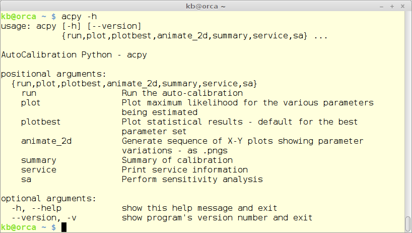
Note that the released version of ACPy might not compare 100% to the above figure.
ACPy usage
ACPy is a python wrapper around a number of individual python modules. It only provides common configuration between the modules and set up infrastructure. Each of the individual modules - described below - handles their own usage and help. The very modular way ACPy is implemented makes it easy to add new functionally to the main program.
All execution of ACPY commands is done via the ‘acpy’ command wrapper - see the figure above.
Main configuration file
ACPy is configured via a xml formatted file. The example below is from the Northern North Sea annual standard set-up. The configuration file contains 5 different sections:
- transports - how are results communicated and stored
- executable path - the full path to the executable - in this case GOTM
- setup path - that path to the basic set-up
- parameters - list of parameters to use in the calibration
- observations - list of observation files - in the format shown further down
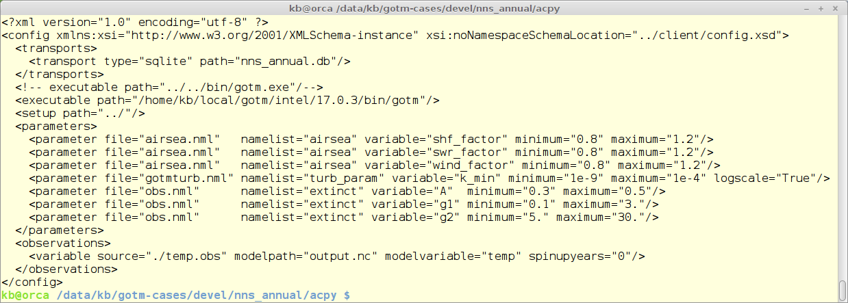
The configuration has optimized for 7 parameters in the model (the 8th is a dummy variable for testing). The y-axis is the maximum likelihood value and the x-axes show the span for the different parameters. ACPy supports logaritmic parameters - as the specification for k_min shows.
Parameters to optimize can specified via Fortran namelist or YAML-formatted syntax.
Database file
The autocalibration module - see the ‘run’ module - with the configuration above creates a SQLite formatted database with the results of the autocalibration tools. The specific name of this file is specified in the .xml configuration file. Most other modules with use the database file for futher processing.
Observation file format
Observations in ACPy are read in from simple ASCII files with one variable in each file. The observation files are listed in the main configuration file and links the file to a output file and model variable. The format is very simple as seen in the figure below. Each observation consists of a time-stamp and a depth (measure from the surface).
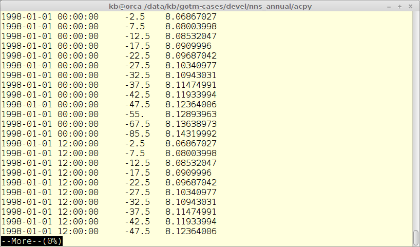
The observations are used to calculate the maximum likelihood function on which the auto-calibration is based.
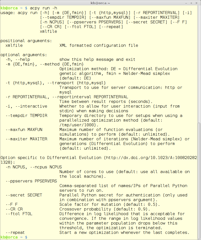
The ‘run’ module
The run module is the workhorse of ACPy and does the actual auto-calibration. The run command takes a large number of commandline parameters of which one is mandatory - the .xml configuration file - and all others are optional.
An overview of all the parameters can be shown using this command:
acpy run -h
with this result:
The ‘plot’ module
The plot module gives a graphical overview of the calibration process. A sub-plot is created for each of the parameters from the configuration file. On the x-axis the sub-plots has the range for the parameter in question - and on the y-axis the maximum likelihood value. An example if provided further down.
acpy plot -h
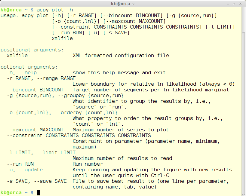
The plot module also takes a relative large number of parameters. Here only one will be mentioned - -u. Giving this option the plot will be autoomatically updated as new results are stored in the database file.
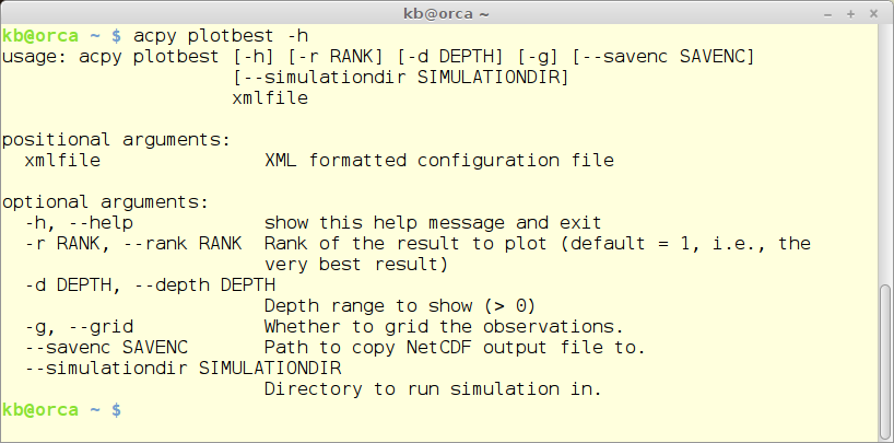
The ‘plotbest’ module
The plotbest module re-runs a specific run - default the best one - and provides 3 plots and calculates some statistical parameters.
acpy plotbest -h
The ‘animate_2d’ module
acpy animate_2d -h
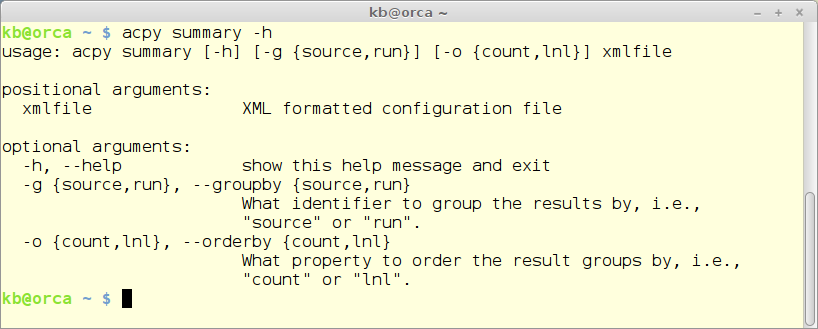
The ‘summary’ module
acpy summary -h